机器学习的工作原理是通过使用算法从数据中学习知识,然后对现实世界中的事件做出预测或决策。它使用大量的数据来“训练”模型,通过不同的算法从数据中学习如何完成任务。与传统的硬编码软件程序不同,机器学习模型可以通过新的数据不断自我修正和改进。
机器学习的优势在于其能够从越来越多的输入数据中学习,并给出数据驱动的概率预测。这使得机器学习在处理复杂数据和做出准确预测方面具有显著优势。此外,机器学习在许多领域都有广泛应用,包括金融服务、物流、供应链、边缘计算等。
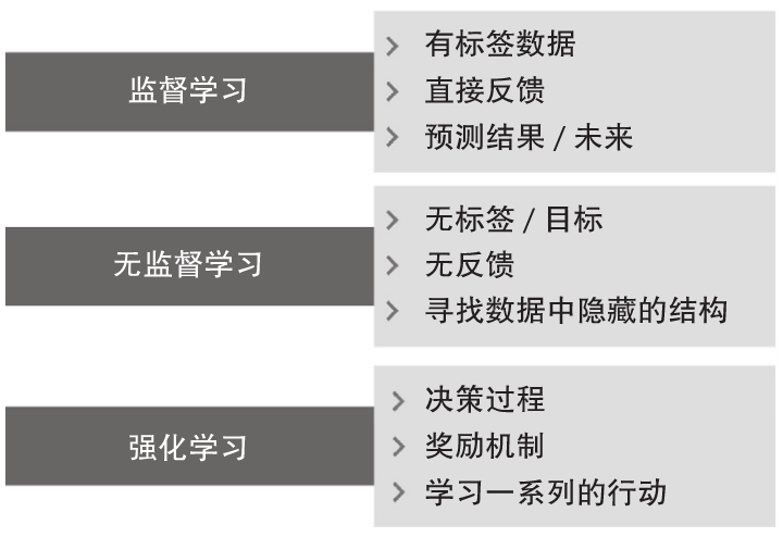
机器学习一般分为三种类型:监督学习、无监督学习和强化学习。
下面我们用机器学习和统计学中一个经典的数据集开始机器学习之旅:鸢尾花(Iris)数据集,它包含在 scikit-learn 的 datasets 模块中。
我们将基于这个数据集完成一个简单的机器学习应用,构建第一个模型。假设有一名植物学爱好者对发现的鸢尾花的品种很感兴趣。他收集了每朵鸢尾花的一些测量数据:花瓣的长度和宽度,花萼的长度和宽度,测量结果的单位都是厘米。另外还有一些已知品种的的测量数据,这些已知的测量数据已经被植物学专家鉴定为属于鸢尾花 setosa、 versicolor 或 virginica 三个品种之一。
因为我们有已知品种的鸢尾花的测量数据,所以这是一个监督学习问题。

在这个问题中, 我们要在多个选项中预测其中一个(鸢尾花的品种),这是一个分类(classification)问题的示例。可能的输出(鸢尾花的不同品种)叫作类别(class)。数据集中的每朵鸢尾花都属于三个类别之一,所以这是一个三分类问题。单个数据点(一朵鸢尾花)的预期输出是这朵花的品种。对于一个数据点来说,它的品种叫作标签(label)。看一下代码示例(看注释):
# 从scikit-learn 的 datasets 模块中导入鸢尾花(Iris)数据集
from sklearn.datasets import load_iris# 加载数据集,返回一个 Bunch 对象,与字典非常相似,里面包含键和值
iris_dataset = load_iris()
print("Keys of iris_dataset: \n{}".format(iris_dataset.keys()))
# 输出内容:
# Keys of iris_dataset:
# dict_keys(['data', 'target', 'frame', 'target_names', 'DESCR', 'feature_names', 'filename', 'data_module'])# DESCR 键对应的值是数据集的简要说明
print(iris_dataset['DESCR'][:193] + "\n...")# target_names 键对应的值是一个字符串数组,里面包含我们要预测的花的品种
# 下面输出:Target names: ['setosa' 'versicolor' 'virginica']
print("Target names: {}".format(iris_dataset['target_names']))# feature_names 键对应的值是一个字符串列表,对每一个特征进行了说明
# 下面输出:
# Feature names:
# ['sepal length (cm)', 'sepal width (cm)', 'petal length (cm)', 'petal width (cm)']
print("Feature names: \n{}".format(iris_dataset['feature_names']))# 数据集的数据包含在 target 和 data 字段中。data 里面是花萼长度、花萼宽度、花瓣长度、花瓣宽度的测量数据,
# 格式为 NumPy 数组:Type of data: <class 'numpy.ndarray'>
print("Type of data: {}".format(type(iris_dataset['data'])))# data 数组的每一行对应一朵花,列代表每朵花的四个测量数据
# Shape of data: (150, 4)
print("Shape of data: {}".format(iris_dataset['data'].shape))
从最最后data的输出可以看出,数组中包含 150 朵不同的花的测量数据。前面说过,机器学习中的个体叫作样本(sample),其属性叫作特征(feature)。data 数组的形状(shape)是样本数乘以特征数。这是 scikit-learn 中的约定,你的数据形状应始终遵循这个约定。下面给出前 5 个样 本的特征数值:
# 从scikit-learn 的 datasets 模块中导入鸢尾花(Iris)数据集
from sklearn.datasets import load_iris# 加载数据集,返回一个 Bunch 对象,与字典非常相似,里面包含键和值
iris_dataset = load_iris()
print("Keys of iris_dataset: \n{}".format(iris_dataset.keys()))
# 输出内容:
# Keys of iris_dataset:
# dict_keys(['data', 'target', 'frame', 'target_names', 'DESCR', 'feature_names', 'filename', 'data_module'])# DESCR 键对应的值是数据集的简要说明
print(iris_dataset['DESCR'][:193] + "\n...")# target_names 键对应的值是一个字符串数组,里面包含我们要预测的花的品种
# 下面输出:Target names: ['setosa' 'versicolor' 'virginica']
print("Target names: {}".format(iris_dataset['target_names']))# feature_names 键对应的值是一个字符串列表,对每一个特征进行了说明
# 下面输出:
# Feature names:
# ['sepal length (cm)', 'sepal width (cm)', 'petal length (cm)', 'petal width (cm)']
print("Feature names: \n{}".format(iris_dataset['feature_names']))# 数据集的数据包含在 target 和 data 字段中。data 里面是花萼长度、花萼宽度、花瓣长度、花瓣宽度的测量数据,
# 格式为 NumPy 数组:Type of data: <class 'numpy.ndarray'>
print("Type of data: {}".format(type(iris_dataset['data'])))# data 数组的每一行对应一朵花,列代表每朵花的四个测量数据
# Shape of data: (150, 4)
print("Shape of data: {}".format(iris_dataset['data'].shape))# 前5个样本的特征数值
print("First five rows of data:\n{}".format(iris_dataset['data'][:5]))
上面代码中最后一行输出前5个样本特征数值:
[[5.1 3.5 1.4 0.2]
[4.9 3. 1.4 0.2]
[4.7 3.2 1.3 0.2]
[4.6 3.1 1.5 0.2]
[5. 3.6 1.4 0.2]]
从数据中可以看出,前 5 朵花的花瓣宽度都是 0.2cm,第一朵花的花萼最长,是 5.1cm。 target 数组包含的是测量过的每朵花的品种,也是一个 NumPy 数组:
# 从scikit-learn 的 datasets 模块中导入鸢尾花(Iris)数据集
from sklearn.datasets import load_iris# 加载数据集,返回一个 Bunch 对象,与字典非常相似,里面包含键和值
iris_dataset = load_iris()
print("Keys of iris_dataset: \n{}".format(iris_dataset.keys()))
# 输出内容:
# Keys of iris_dataset:
# dict_keys(['data', 'target', 'frame', 'target_names', 'DESCR', 'feature_names', 'filename', 'data_module'])# DESCR 键对应的值是数据集的简要说明
print(iris_dataset['DESCR'][:193] + "\n...")# target_names 键对应的值是一个字符串数组,里面包含我们要预测的花的品种
# 下面输出:Target names: ['setosa' 'versicolor' 'virginica']
print("Target names: {}".format(iris_dataset['target_names']))# feature_names 键对应的值是一个字符串列表,对每一个特征进行了说明
# 下面输出:
# Feature names:
# ['sepal length (cm)', 'sepal width (cm)', 'petal length (cm)', 'petal width (cm)']
print("Feature names: \n{}".format(iris_dataset['feature_names']))# 数据集的数据包含在 target 和 data 字段中。data 里面是花萼长度、花萼宽度、花瓣长度、花瓣宽度的测量数据,
# 格式为 NumPy 数组:Type of data: <class 'numpy.ndarray'>
print("Type of data: {}".format(type(iris_dataset['data'])))# data 数组的每一行对应一朵花,列代表每朵花的四个测量数据
# Shape of data: (150, 4)
print("Shape of data: {}".format(iris_dataset['data'].shape))# 前5个样本的特征数值
print("First five rows of data:\n{}".format(iris_dataset['data'][:5]))# target 数组包含的是测量过的每朵花的品种,也是一个 NumPy 数组:
# 输出:Type of target: <class 'numpy.ndarray'>
print("Type of target: {}".format(type(iris_dataset['target'])))# target 是一维数组,每朵花对应其中一个数据
print("Shape of target: {}".format(iris_dataset['target'].shape))# 品种被转换成从 0 到 2 的整数
print("Target:\n{}".format(iris_dataset['target']))
以上代码Target输出:
Target:
[0 0 0 0 0 0 0 0 0 0 0 0 0 0 0 0 0 0 0 0 0 0 0 0 0 0 0 0 0 0 0 0 0 0 0 0 0
0 0 0 0 0 0 0 0 0 0 0 0 0 1 1 1 1 1 1 1 1 1 1 1 1 1 1 1 1 1 1 1 1 1 1 1 1
1 1 1 1 1 1 1 1 1 1 1 1 1 1 1 1 1 1 1 1 1 1 1 1 1 1 2 2 2 2 2 2 2 2 2 2 2
2 2 2 2 2 2 2 2 2 2 2 2 2 2 2 2 2 2 2 2 2 2 2 2 2 2 2 2 2 2 2 2 2 2 2 2 2
2 2]
上述数字的代表含义由 iris['target_names'] 数组给出:0 代表 setosa,1 代表 versicolor, 2 代表 virginica。
训练数据与测试数据
我们想要利用这些数据构建一个机器学习模型,用于预测新测量的鸢尾花的品种。但在将模型应用于新的测量数据之前,我们需要知道模型是否有效,也就是说,我们是否应该相信它的预测结果。 不幸的是,我们不能将用于构建模型的数据用于评估模型。因为我们的模型会一直记住整个训练集,所以对于训练集中的任何数据点总会预测正确的标签。这种“记忆”无法告诉我们模型的泛化(generalize)能力如何(换句话说,在新数据上能否正确预测)。
我们要用新数据来评估模型的性能。新数据是指模型之前没有见过的数据,而我们有这些新数据的标签。通常的做法是将收集好的带标签数据(此例中是 150 朵花的测量数据) 分成两部分。一部分数据用于构建机器学习模型,叫作训练数据(training data)或训练集(training set)。其余的数据用来评估模型性能,叫作测试数据(test data)、测试集(test set)或留出集(hold-out set)。
scikit-learn 中的 train_test_split 函数可以打乱数据集并进行拆分:将 75% 的行数据及对应标签作为训练集,剩下 25% 的数据及其标签作为测试集。训练集与测试集的分配比例可以是随意的,但使用 25% 的数据作为测试集是很好的经验法则。
scikit-learn 中的数据用大写的 X 表示,标签用小写的 y 表示。类似于数学标准公式 f(x)=y ,其中 x 是函数的输入,y 是输出。用大写的 X 是因为数据是 一个二维数组(矩阵),用小写的 y 是因为目标是一个一维数组(向量),这也是数学中的约定。
观察数据
构建机器学习模型之前,最好检查一下数据,看看是否有异常值和特殊值。检查数据的最佳方法之一就是将其可视化。例如绘制散点图(scatter plot)。 数据散点图将一个特征作为 x 轴,另一个特征作为 y 轴,将每一个数据点绘制为图上的一 个点。不幸的是,计算机屏幕只有两个维度,所以我们一次只能绘制两个特征(也可能是 3 个)。用这种方法难以对多于 3 个特征的数据集作图。解决这个问题的一种方法是绘制散点图矩阵(pair plot),从而可以两两查看所有的特征。如果特征数不多的话,比如我们这里有 4 个,这种方法是很合理的。但是我们要注意,散点图矩阵无法同时显示所有特征之间的关系,所以这种可视化方法可能无法展示数据的某些有趣内容。
import numpy as np
import pandas as pd
import matplotlib.pyplot as plt
import mglearn
# 从scikit-learn 的 datasets 模块中导入鸢尾花(Iris)数据集
from sklearn.datasets import load_iris
# 导入train_test_split函数
from sklearn.model_selection import train_test_split# 加载数据集,返回一个 Bunch 对象,与字典非常相似,里面包含键和值
iris_dataset = load_iris()
print("Keys of iris_dataset: \n{}".format(iris_dataset.keys()))
# 输出内容:
# Keys of iris_dataset:
# dict_keys(['data', 'target', 'frame', 'target_names', 'DESCR', 'feature_names', 'filename', 'data_module'])# DESCR 键对应的值是数据集的简要说明
print(iris_dataset['DESCR'][:193] + "\n...")# target_names 键对应的值是一个字符串数组,里面包含我们要预测的花的品种
# 下面输出:Target names: ['setosa' 'versicolor' 'virginica']
print("Target names: {}".format(iris_dataset['target_names']))# feature_names 键对应的值是一个字符串列表,对每一个特征进行了说明
# 下面输出:
# Feature names:
# ['sepal length (cm)', 'sepal width (cm)', 'petal length (cm)', 'petal width (cm)']
print("Feature names: \n{}".format(iris_dataset['feature_names']))# 数据集的数据包含在 target 和 data 字段中。data 里面是花萼长度、花萼宽度、花瓣长度、花瓣宽度的测量数据,
# 格式为 NumPy 数组:Type of data: <class 'numpy.ndarray'>
print("Type of data: {}".format(type(iris_dataset['data'])))# data 数组的每一行对应一朵花,列代表每朵花的四个测量数据
# Shape of data: (150, 4)
print("Shape of data: {}".format(iris_dataset['data'].shape))# 前5个样本的特征数值
print("First five rows of data:\n{}".format(iris_dataset['data'][:5]))# target 数组包含的是测量过的每朵花的品种,也是一个 NumPy 数组:
# 输出:Type of target: <class 'numpy.ndarray'>
print("Type of target: {}".format(type(iris_dataset['target'])))# target 是一维数组,每朵花对应其中一个数据
print("Shape of target: {}".format(iris_dataset['target'].shape))# 品种被转换成从 0 到 2 的整数
print("Target:\n{}".format(iris_dataset['target']))#========================================================================
# 拆分数据集为训练集、测试集
# train_test_split 函数的输出为 X_train、X_test、y_train 和 y_test,
# 它们都是NumPy数组。X_train 包含 75% 的行数据,X_test 包含剩下的 25%
X_train, X_test, y_train, y_test = train_test_split(iris_dataset['data'], iris_dataset['target'], random_state=0)# 输出:
# X_train shape: (112, 4)
# y_train shape: (112,)
print("X_train shape: {}".format(X_train.shape))
print("y_train shape: {}".format(y_train.shape))# 输出:
# X_test shape: (38, 4)
# y_test shape: (38,)
print("X_test shape: {}".format(X_test.shape))
print("y_test shape: {}".format(y_test.shape))# ================================================================
# 观察数据
# 利用X_train中的数据创建DataFrame
# 利用iris_dataset.feature_names中的字符串对数据列进行标记
iris_dataframe = pd.DataFrame(X_train, columns=iris_dataset.feature_names)
# 利用DataFrame创建散点图矩阵,按y_train着色
grr = pd.plotting.scatter_matrix(iris_dataframe, c=y_train, figsize=(15, 15), marker='o', hist_kwds={'bins': 20}, s=60, alpha=.8, cmap=mglearn.cm3)
plt.show()
输出训练集中特征的散点图矩阵:

数据点的颜色与鸢尾花的品种相对应。为了绘制这张图,我们首先将 NumPy 数组转换成 pandas DataFrame。pandas 有一个绘制散点图矩阵的函数,叫作 scatter_matrix。矩阵的对角线是每个特征的直方图。从图中可以看出,利用花瓣和花萼的测量数据基本可以将三个类别区分开。这说明机器学习模型很可能可以学会区分它们。
构建第一个模型:k近邻算法
scikit-learn 中有许多可用的分类算法。 这里我们用的是 k 近邻分类器,此模型只需要保存训练集即可。要对一个新的数据点做出预测,算法会在训练集中寻找与这个新数据点距离最近的数据点,然后将找到的数据点的标签赋值给这个新数据点。
k 近邻算法中 k 的含义是,可以考虑训练集中与新数据点最近的任意 k 个邻居(比如说,距离最近的 3 个或 5 个邻居),而不是只考虑最近的那一个。然后,我们可以用这些邻居中数量最多的类别做出预测。现在我们只考虑 一个邻居的情况。
scikit-learn 中所有的机器学习模型都在各自的类中实现,这些类被称为 Estimator 类。k 近邻分类算法是在 neighbors 模块的 KNeighborsClassifier 类中实现的。我们需要将这个类实例化为一个对象,然后才能使用这个模型。这时我们需要设置模型的参数。 KNeighborsClassifier 最重要的参数就是邻居的数目k,这里我们设为 1:
from sklearn.neighbors import KNeighborsClassifier
knn = KNeighborsClassifier(n_neighbors=1)
knn 对象对算法进行了封装,既包括用训练数据构建模型的算法,也包括对新数据点进行预测的算法。它还包括算法从训练数据中提取的信息。对于 KNeighborsClassifier 来说, 里面只保存了训练集。 想要基于训练集来构建模型,需要调用 knn 对象的 fit 方法,输入参数为 X_train 和 y_ train,二者都是 NumPy 数组,前者包含训练数据,后者包含相应的训练标签:
import numpy as np
import pandas as pd
import matplotlib.pyplot as plt
import mglearn
# 从scikit-learn 的 datasets 模块中导入鸢尾花(Iris)数据集
from sklearn.datasets import load_iris
# 导入train_test_split函数
from sklearn.model_selection import train_test_split# 加载数据集,返回一个 Bunch 对象,与字典非常相似,里面包含键和值
iris_dataset = load_iris()
print("Keys of iris_dataset: \n{}".format(iris_dataset.keys()))
# 输出内容:
# Keys of iris_dataset:
# dict_keys(['data', 'target', 'frame', 'target_names', 'DESCR', 'feature_names', 'filename', 'data_module'])# DESCR 键对应的值是数据集的简要说明
print(iris_dataset['DESCR'][:193] + "\n...")# target_names 键对应的值是一个字符串数组,里面包含我们要预测的花的品种
# 下面输出:Target names: ['setosa' 'versicolor' 'virginica']
print("Target names: {}".format(iris_dataset['target_names']))# feature_names 键对应的值是一个字符串列表,对每一个特征进行了说明
# 下面输出:
# Feature names:
# ['sepal length (cm)', 'sepal width (cm)', 'petal length (cm)', 'petal width (cm)']
print("Feature names: \n{}".format(iris_dataset['feature_names']))# 数据集的数据包含在 target 和 data 字段中。data 里面是花萼长度、花萼宽度、花瓣长度、花瓣宽度的测量数据,
# 格式为 NumPy 数组:Type of data: <class 'numpy.ndarray'>
print("Type of data: {}".format(type(iris_dataset['data'])))# data 数组的每一行对应一朵花,列代表每朵花的四个测量数据
# Shape of data: (150, 4)
print("Shape of data: {}".format(iris_dataset['data'].shape))# 前5个样本的特征数值
print("First five rows of data:\n{}".format(iris_dataset['data'][:5]))# target 数组包含的是测量过的每朵花的品种,也是一个 NumPy 数组:
# 输出:Type of target: <class 'numpy.ndarray'>
print("Type of target: {}".format(type(iris_dataset['target'])))# target 是一维数组,每朵花对应其中一个数据
print("Shape of target: {}".format(iris_dataset['target'].shape))# 品种被转换成从 0 到 2 的整数
print("Target:\n{}".format(iris_dataset['target']))#========================================================================
# 拆分数据集为训练集、测试集
# train_test_split 函数的输出为 X_train、X_test、y_train 和 y_test,
# 它们都是NumPy数组。X_train 包含 75% 的行数据,X_test 包含剩下的 25%
X_train, X_test, y_train, y_test = train_test_split(iris_dataset['data'], iris_dataset['target'], random_state=0)# 输出:
# X_train shape: (112, 4)
# y_train shape: (112,)
print("X_train shape: {}".format(X_train.shape))
print("y_train shape: {}".format(y_train.shape))# 输出:
# X_test shape: (38, 4)
# y_test shape: (38,)
print("X_test shape: {}".format(X_test.shape))
print("y_test shape: {}".format(y_test.shape))# ================================================================
# 观察数据
# 利用X_train中的数据创建DataFrame
# 利用iris_dataset.feature_names中的字符串对数据列进行标记
iris_dataframe = pd.DataFrame(X_train, columns=iris_dataset.feature_names)
# 利用DataFrame创建散点图矩阵,按y_train着色
grr = pd.plotting.scatter_matrix(iris_dataframe, c=y_train, figsize=(15, 15), marker='o', hist_kwds={'bins': 20}, s=60, alpha=.8, cmap=mglearn.cm3)
plt.show()# ================================================================
# 调用 knn 对象的 fit 方法基于训练集来构建模型
from sklearn.neighbors import KNeighborsClassifier
knn = KNeighborsClassifier(n_neighbors=1)
knn.fit(X_train, y_train)
fit 方法返回的是 knn 对象本身并做原地修改,因此我们得到了分类器的字符串表示。
KNeighborsClassifier(n_neighbors=1)
从中可以看出构建模型时用到的参数。n_ neighbors=1,这是我们传入的参数。scikit-learn 中的大多数模型都有很多参数,但多用于速度优化或非常特殊的用途。无需关注这个字符串表示中的其他参数。
做出预测
现在我们可以用这个模型对新数据进行预测了,我们可能并不知道这些新数据的正确标签。假如,我们在野外发现了一朵鸢尾花,花萼长 5cm 宽 2.9cm,花瓣长 1cm 宽 0.3cm。这朵鸢尾花属于哪个品种?我们将这些数据放在一个 NumPy 数组中,数组形状为样本数(1)乘以特征数(4),然后调用knn 对象的 predict 方法来进行预测:
import numpy as np
import pandas as pd
import matplotlib.pyplot as plt
import mglearn
# 从scikit-learn 的 datasets 模块中导入鸢尾花(Iris)数据集
from sklearn.datasets import load_iris
# 导入train_test_split函数
from sklearn.model_selection import train_test_split# 加载数据集,返回一个 Bunch 对象,与字典非常相似,里面包含键和值
iris_dataset = load_iris()
print("Keys of iris_dataset: \n{}".format(iris_dataset.keys()))
# 输出内容:
# Keys of iris_dataset:
# dict_keys(['data', 'target', 'frame', 'target_names', 'DESCR', 'feature_names', 'filename', 'data_module'])# DESCR 键对应的值是数据集的简要说明
print(iris_dataset['DESCR'][:193] + "\n...")# target_names 键对应的值是一个字符串数组,里面包含我们要预测的花的品种
# 下面输出:Target names: ['setosa' 'versicolor' 'virginica']
print("Target names: {}".format(iris_dataset['target_names']))# feature_names 键对应的值是一个字符串列表,对每一个特征进行了说明
# 下面输出:
# Feature names:
# ['sepal length (cm)', 'sepal width (cm)', 'petal length (cm)', 'petal width (cm)']
print("Feature names: \n{}".format(iris_dataset['feature_names']))# 数据集的数据包含在 target 和 data 字段中。data 里面是花萼长度、花萼宽度、花瓣长度、花瓣宽度的测量数据,
# 格式为 NumPy 数组:Type of data: <class 'numpy.ndarray'>
print("Type of data: {}".format(type(iris_dataset['data'])))# data 数组的每一行对应一朵花,列代表每朵花的四个测量数据
# Shape of data: (150, 4)
print("Shape of data: {}".format(iris_dataset['data'].shape))# 前5个样本的特征数值
print("First five rows of data:\n{}".format(iris_dataset['data'][:5]))# target 数组包含的是测量过的每朵花的品种,也是一个 NumPy 数组:
# 输出:Type of target: <class 'numpy.ndarray'>
print("Type of target: {}".format(type(iris_dataset['target'])))# target 是一维数组,每朵花对应其中一个数据
print("Shape of target: {}".format(iris_dataset['target'].shape))# 品种被转换成从 0 到 2 的整数
print("Target:\n{}".format(iris_dataset['target']))#========================================================================
# 拆分数据集为训练集、测试集
# train_test_split 函数的输出为 X_train、X_test、y_train 和 y_test,
# 它们都是NumPy数组。X_train 包含 75% 的行数据,X_test 包含剩下的 25%
X_train, X_test, y_train, y_test = train_test_split(iris_dataset['data'], iris_dataset['target'], random_state=0)# 输出:
# X_train shape: (112, 4)
# y_train shape: (112,)
print("X_train shape: {}".format(X_train.shape))
print("y_train shape: {}".format(y_train.shape))# 输出:
# X_test shape: (38, 4)
# y_test shape: (38,)
print("X_test shape: {}".format(X_test.shape))
print("y_test shape: {}".format(y_test.shape))# ================================================================
# 观察数据
# 利用X_train中的数据创建DataFrame
# 利用iris_dataset.feature_names中的字符串对数据列进行标记
iris_dataframe = pd.DataFrame(X_train, columns=iris_dataset.feature_names)
# 利用DataFrame创建散点图矩阵,按y_train着色
grr = pd.plotting.scatter_matrix(iris_dataframe, c=y_train, figsize=(15, 15), marker='o', hist_kwds={'bins': 20}, s=60, alpha=.8, cmap=mglearn.cm3)
plt.show()# ================================================================
# 调用 knn 对象的 fit 方法基于训练集来构建模型
from sklearn.neighbors import KNeighborsClassifier
knn = KNeighborsClassifier(n_neighbors=1)
knn.fit(X_train, y_train)# ================================================================
# 对新数据做出预测,新发现了一朵鸢尾花,花萼长 5cm 宽 2.9cm,花瓣长 1cm 宽 0.3cm,
# 用上面训练出的模型来预测它属于哪个品种
X_new = np.array([[5, 2.9, 1, 0.3]])
print("X_new.shape: {}".format(X_new.shape))# 调用 knn 对象的 predict 方法来进行预测
prediction = knn.predict(X_new)
print("Prediction: {}".format(prediction))
print("Predicted target name: {}".format(iris_dataset['target_names'][prediction]))
# 预测结果输出如下:
# Prediction: [0]
# Predicted target name: ['setosa']
预测结果输出如下:
Prediction: [0]
Predicted target name: ['setosa']]
根据模型的预测,这朵新的鸢尾花属于类别 0,也就是说它属于 setosa 品种。但我们怎么知道能否相信这个模型呢?我们并不知道这个样本的实际品种,这也是我们构建模型的重点,评估模型。
评估模型
这里需要用到之前创建的测试集。这些数据没有用于构建模型,但我们知道测试集中每朵鸢尾花的实际品种。 因此,我们可以对测试数据中的每朵鸢尾花进行预测,并将预测结果与标签(已知的品 种)进行对比。我们可以通过计算精度(accuracy)来衡量模型的优劣,精度就是品种预测正确的花所占的比例:
import numpy as np
import pandas as pd
import matplotlib.pyplot as plt
import mglearn
# 从scikit-learn 的 datasets 模块中导入鸢尾花(Iris)数据集
from sklearn.datasets import load_iris
# 导入train_test_split函数
from sklearn.model_selection import train_test_split# 加载数据集,返回一个 Bunch 对象,与字典非常相似,里面包含键和值
iris_dataset = load_iris()
print("Keys of iris_dataset: \n{}".format(iris_dataset.keys()))
# 输出内容:
# Keys of iris_dataset:
# dict_keys(['data', 'target', 'frame', 'target_names', 'DESCR', 'feature_names', 'filename', 'data_module'])# DESCR 键对应的值是数据集的简要说明
print(iris_dataset['DESCR'][:193] + "\n...")# target_names 键对应的值是一个字符串数组,里面包含我们要预测的花的品种
# 下面输出:Target names: ['setosa' 'versicolor' 'virginica']
print("Target names: {}".format(iris_dataset['target_names']))# feature_names 键对应的值是一个字符串列表,对每一个特征进行了说明
# 下面输出:
# Feature names:
# ['sepal length (cm)', 'sepal width (cm)', 'petal length (cm)', 'petal width (cm)']
print("Feature names: \n{}".format(iris_dataset['feature_names']))# 数据集的数据包含在 target 和 data 字段中。data 里面是花萼长度、花萼宽度、花瓣长度、花瓣宽度的测量数据,
# 格式为 NumPy 数组:Type of data: <class 'numpy.ndarray'>
print("Type of data: {}".format(type(iris_dataset['data'])))# data 数组的每一行对应一朵花,列代表每朵花的四个测量数据
# Shape of data: (150, 4)
print("Shape of data: {}".format(iris_dataset['data'].shape))# 前5个样本的特征数值
print("First five rows of data:\n{}".format(iris_dataset['data'][:5]))# target 数组包含的是测量过的每朵花的品种,也是一个 NumPy 数组:
# 输出:Type of target: <class 'numpy.ndarray'>
print("Type of target: {}".format(type(iris_dataset['target'])))# target 是一维数组,每朵花对应其中一个数据
print("Shape of target: {}".format(iris_dataset['target'].shape))# 品种被转换成从 0 到 2 的整数
print("Target:\n{}".format(iris_dataset['target']))#========================================================================
# 拆分数据集为训练集、测试集
# train_test_split 函数的输出为 X_train、X_test、y_train 和 y_test,
# 它们都是NumPy数组。X_train 包含 75% 的行数据,X_test 包含剩下的 25%
X_train, X_test, y_train, y_test = train_test_split(iris_dataset['data'], iris_dataset['target'], random_state=0)# 输出:
# X_train shape: (112, 4)
# y_train shape: (112,)
print("X_train shape: {}".format(X_train.shape))
print("y_train shape: {}".format(y_train.shape))# 输出:
# X_test shape: (38, 4)
# y_test shape: (38,)
print("X_test shape: {}".format(X_test.shape))
print("y_test shape: {}".format(y_test.shape))# ================================================================
# 观察数据
# 利用X_train中的数据创建DataFrame
# 利用iris_dataset.feature_names中的字符串对数据列进行标记
iris_dataframe = pd.DataFrame(X_train, columns=iris_dataset.feature_names)
# 利用DataFrame创建散点图矩阵,按y_train着色
grr = pd.plotting.scatter_matrix(iris_dataframe, c=y_train, figsize=(15, 15), marker='o', hist_kwds={'bins': 20}, s=60, alpha=.8, cmap=mglearn.cm3)
plt.show()# ================================================================
# 调用 knn 对象的 fit 方法基于训练集来构建模型
from sklearn.neighbors import KNeighborsClassifier
knn = KNeighborsClassifier(n_neighbors=1)
knn.fit(X_train, y_train)# ================================================================
# 对新数据做出预测,新发现了一朵鸢尾花,花萼长 5cm 宽 2.9cm,花瓣长 1cm 宽 0.3cm,
# 用上面训练出的模型来预测它属于哪个品种
X_new = np.array([[5, 2.9, 1, 0.3]])
print("X_new.shape: {}".format(X_new.shape))# 调用 knn 对象的 predict 方法来进行预测
prediction = knn.predict(X_new)
print("Prediction: {}".format(prediction))
print("Predicted target name: {}".format(iris_dataset['target_names'][prediction]))
# 预测结果输出如下:
# Prediction: [0]
# Predicted target name: ['setosa']# ================================================================================
# 用测试集评估模型
y_pred = knn.predict(X_test)
print("Test set predictions:\n {}".format(y_pred))
# 评估精度
print("Test set score: {:.2f}".format(np.mean(y_pred == y_test)))
模型评估结果输出:
Test set predictions:
[2 1 0 2 0 2 0 1 1 1 2 1 1 1 1 0 1 1 0 0 2 1 0 0 2 0 0 1 1 0 2 1 0 2 2 1 0 2]
Test set score: 0.97
对于这个模型来说,测试集的精度约为 0.97,也就是说,对于测试集中的鸢尾花,我们的预测有 97% 是正确的。根据一些数学假设,对于新的鸢尾花,可以认为我们的模型预测结果有 97% 都是正确的。高精度意味着模型足够可信,可以使用。在后续我们将学习提高性能的方法,以及模型调参时的注意事项。